CSE168 final project

For the final project of Ravi Ramamoorthi's excellent CSE168, my partner Kevin Wu (GitHub) and I decided to extend our homework 4 renderer (which is derived from instructor-provided starter code that uses Intel Embree) to render volumetric data. If time allowed, we also wanted to combine our renderer with a physical smoke simulation, in line with "Visual Simulation of Smoke" (2001).

Ultimately, we were able to create a decently fast volume renderer modeling light absorption, in-scattering, and out-scattering, as well as intersecting volumes with various properties. In particular, we used a technique known as delta tracking to execute the scattering tests. Unfortunately, we were not able to get our physical simulation working well, although we tested the framework using non-physically-based animations to create amusing videos.

Preliminary investigation using Perlin noise

There are at least two ways we could approach the rendering: ray marching, which involves stepping the ray through the volume in small units; and using our existing ray tracing framework, but sampling the volume along the ray. We decided to go with the second approach because it would involve the least modification to our existing code, and would probably be faster.

As an early test, we took the Cornell box scene and added a cylinder of Perlin noise to the center. The value of the noise at a given point is, conceptually, the density of smoke at that point. We then modeled the absorption of light by sampling the noise a hundred times along the ray, and used an exponential function (with argument equal to the absorption factor $\sigma_a$) to compute the transmittance.

This worked, but was extraordinarily slow.

A large performance improvement was observed by precomputing the Perlin noise in a 3-D grid. It turns out that the expense of computing Perlin noise grows exponentially in the dimension, and we were using a 4-dimensional input (3 spatial, 1 time), so we were spending 95% of execution time in glm::perlin!

We also tried to improve cache locality by indexing the precomputed density field using a space-filling Hilbert curve. But this made the code more complex and the performance was no better; we think this because the density field is already small enough that it fits comfortably in L3.

Easier I/O

We decided to add a simple command to add volumes to the renderer, called volume:

volume <xmin> <ymin> <zmin> <xmax> <ymax> <zmax> <resolution> <r> <g> <b> <absorption coefficient> <expression>

• The first six numbers are the bounds of the volume.
• <resolution> is the size of each voxel.
• <r> <g> <b> are the RGB color of the volume.
• <absorption coefficient> is the absorption coefficient $\sigma_a$ of the material.
• <expression> is a mathematical expression that is evaluated at each point in the volume to give the density. The data type is f32. Supported:
  • Multiplication, addition, subtraction, division, and exponentiation
  • Perlin noise (2, 3, or 4 arguments), clamp, mix, and smoothstep
  • Special functions: abs, sin, cos, tan
  • Comparisons and logical operators

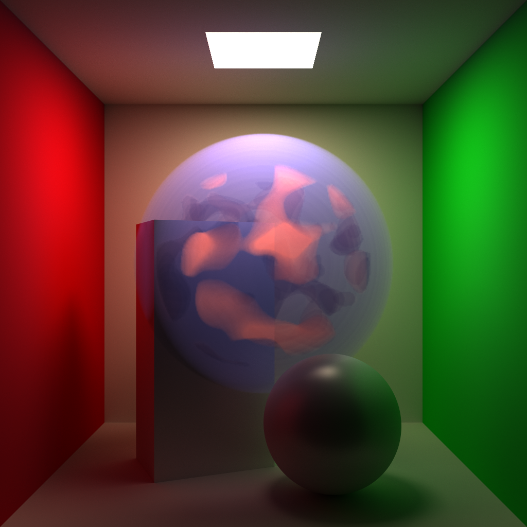
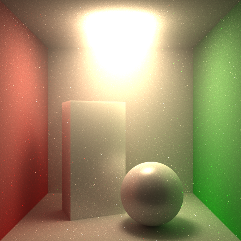
For example, the image at the top of this page is the cornell box scene with two additional volumes:

volume -0.5 0.5 -0.5 0.5 1.5 0.5 0.05 1 0.5 0.5 1 mix(perlin(x*5,y*5,z*5,t*5)>0.3 && length(x,y-1,z) < 0.5, 1, 0)
volume -0.7 0.3 -0.7 0.7 1.7 0.7 0.05 0.15 0.15 0.4 0.2 mix(length(x,y-1,z) < 0.6, 0.2, 0)

This system makes it easy to try new shapes of volumes!

The overall algorithm

We start with the next event estimation (NEE) sampling method built for homework 3 and modify it to account for the volumetric effects. First, we model absorption by scaling the throughput of the ray by (an exponential function of) the amount of material we passed through. This is done by sampling the density at a number of points along the segment. Then, we consider a single scattering event by, essentially, numerically inverting the density CDF. (This will be improved on in the next section.) We draw a ray to the light and compute the contribution using a per-volume phase function, because the reflection is not necessarily isotropic. These values are then summed.

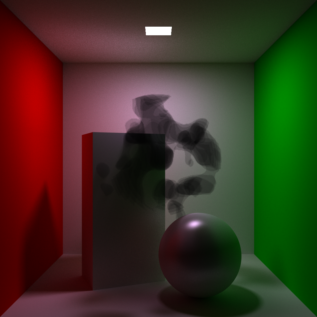
We also test for scattering and absorption when computing indirect lighting. You can see in the first photo above that the purple translucent sphere is reflected in the ceiling and the lower sphere.

We used the Mie phase function for the scattering, described in Ravi's slides:

$p(\cos\theta) = \frac{1}{4\pi}\left(\frac{1}{2}+\frac{z+1}{2}\cdot\left(\frac{1 + \cos\theta}{2}\right)^z\right)$

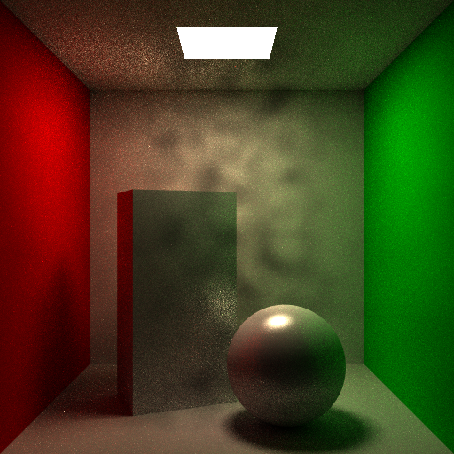
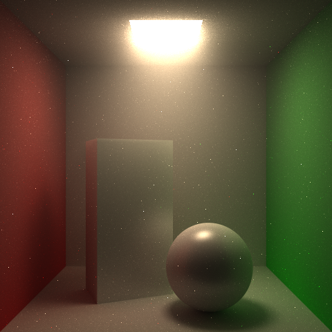
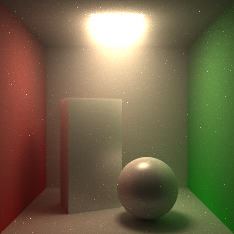
In the first three images in the gallery below, you can see the scattering effects for different values of $z$, $z=2,4,8$.

We now have heterogeneous scattering!

Handling intersecting volumes

Handling intersecting volumes is done by iterating through each volume and finding a scattering event, then choosing the nearest one, if any. This works quite well, especially when the volumes are bounded (so that you can skip volumes that are missed).

Accelerating the scattering code

According to our profiling data, the vast majority of the path tracer execution time was spent calculating the ray scatter position. Rendering an image with smoke was taking twenty times as long as without, and our renderer already isn't terribly optimized. We therefore focused on improving the sampling algorithm.

We then did further research and came across the idea of delta tracking in this paper. The basic idea is that we can start by analytically computing where a scattering event would occur if the volume were homogeneous. In particular, if the scattering coefficient is $\sigma_s$, then the probability of a scattering event occurring at distance $d$ is given by the exponential function $e^{-\sigma_s d}$. We can then sample a random number $u$ from the uniform distribution on $[0, 1]$, and solve for $d$ such that $e^{-\sigma_s d} = u$.

We take $\sigma_s = \max_{p\in\mathbb{R}^3}density(p)$, where $density(p)$ is the density at point $p$. Then, if the algorithm reports a scattering event at $s$, we accept the event with probability $d(s)/\sigma_s$, and otherwise continue to find the next scattering event (or exiting the volume).

This sped up scattering by a factor of 10! Now the renders are only about 1.5x slower than the renders without scattering (and only absorption).

Gallery

Further work

If we had more time, there are several inaccuracies in our renderer that we would like to fix:

• No multiple scattering. This means that the image isn't quite as bright as it should be.
• The rays traced from the scattering points to the light sources are not attenuated.

We also would like to develop a bounding box hierarchy system for the volumes, which would allow us to handle very heterogeneous volumes more efficiently. When you have a volume that has only small areas of high density, the delta tracking scheme requires a large number of intermediate steps before a scatter actually occurs.

Thanks again to Professor Ravi for his excellent lectures and materials, and to our TA, Nithin Raghavan, for his helpful feedback!